Logical Data Model: Logical Normalization

This is a first part of a miniseries underlining the benefits of setting up a proper logical data model (LDM), also known as a semantic data model. Each blog post will show a specific feature of the GoodData LDM, which enables users to create metrics that are both complex and reusable. Additionally, each feature provides extra information about your data to the system and will help you achieve your overall goal.

The GoodData LDM features covered in this miniseries are logical normalization, which is highlighted below; attribute labels; and shared datasets. (For those who are not yet familiar with the basics of an LDM, read this introduction.)

Throughout the series, we will illustrate the functionality via the following task: to create a reusable metric by computing the ratio of order amount on the given report dimensionality to the total order amount for each Region. (This metric is the same one as in my previous article about Multidimensional Analytical Query Language [MAQL]: A Guide to MAQL Metrics Reusability.)

Note: If you want to follow along by building your own LDM, please read Get GoodData.CN and Create a Workspace in the documentation. If you created a workspace and GoodData.CN is running, then execute the following command:

curl http://localhost:3000/api/entities/dataSources \
 -H "Content-Type: application/vnd.gooddata.api+json" \
 -H "Accept: application/vnd.gooddata.api+json" \
 -H "Authorization: Bearer YWRtaW46Ym9vdHN0cmFwOmFkbWluMTIz" \
 -X POST \
 -d '{
     "data": {
         "attributes": {
             "name": "demo-denormalized",
             "url": "jdbc:postgresql://localhost:5432/demo",
             "schema": "demo_denormalized",
             "type": "POSTGRESQL",
             "username": "demouser",
             "password": "demopass"
         },
         "id": "demo-denormalized",
         "type": "dataSource"
     }
 }' | jq .

It connects the demo-denormalized data source, and you should use that data source in your workspace. (In our documentation library, please read the section on how to build a logical data model; this describes how to create an LDM from the connected data source.)

Afterward, you should end up with the LDM pictured below. There are two fact datasets (Order lines and Campaign channels) and a single Date dataset. We will use only the Order lines in this first part.

Relations in the LDM

One crucial property of the datasets is an implied 1:N relation between the primary key (e.g., Order line id) and its attributes (e.g., Customer id, Customer name, etc.). The system doesn’t know anything more, and by default, it assumes that the relations between attributes themselves are all M:N. In other words, it assumes that there are no functional dependencies between attributes, and the dataset is in the third normal form. In reality, this might not be true (e.g., each State belongs to exactly one Region).

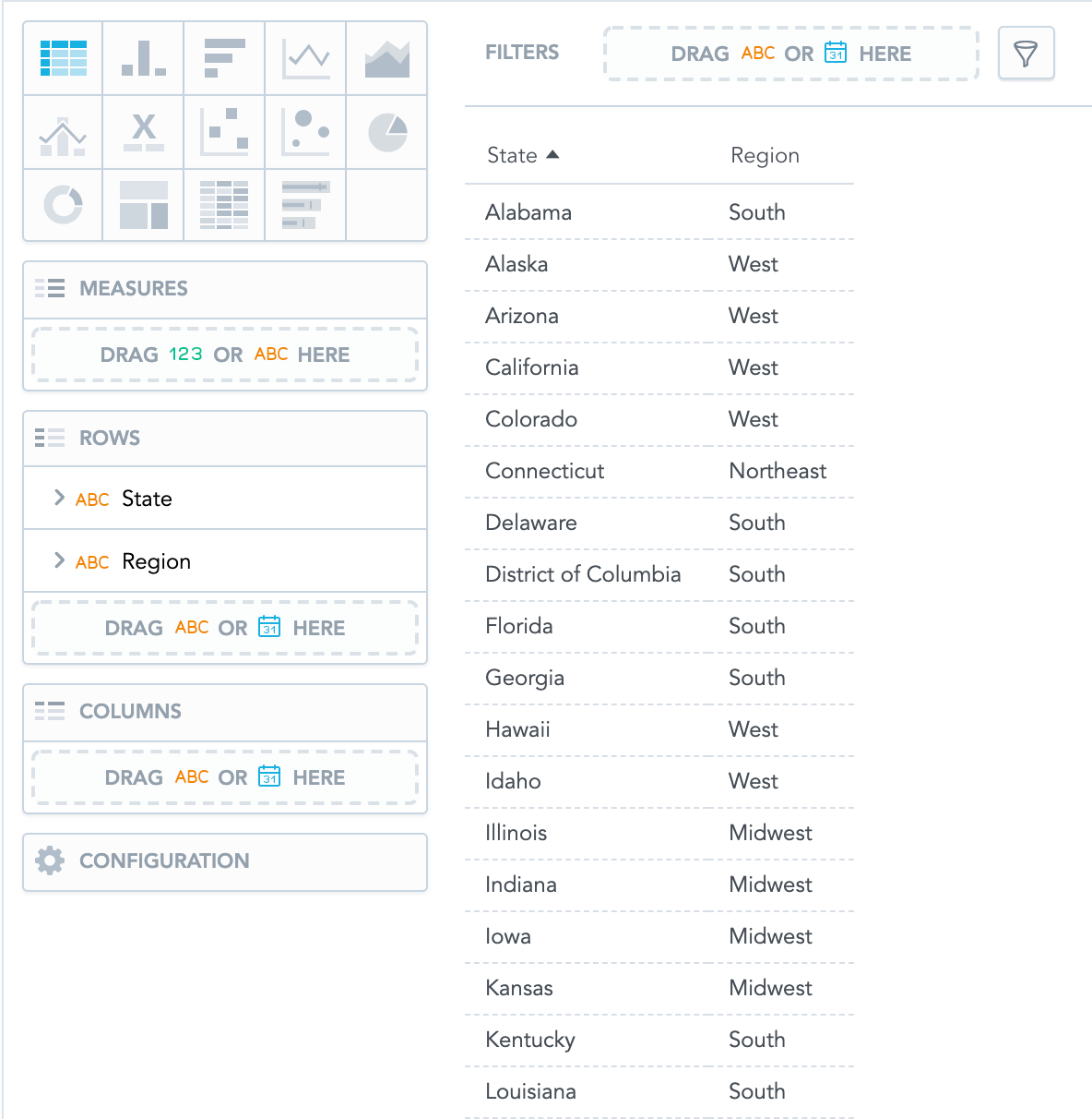
You can check it on the data sample:

The consequences of this “relation” will be revealed later. (Note that the data sample is incomplete, and it is included just for demonstration purposes.)

Metric Definition

Let’s create the reusable metric Order Amount Ratio to Region in MAQL. As described in our guide to MAQL metrics reusability, set the metric format to Percent (rounded).

SELECT (SELECT SUM({fact/price})) / 
(SELECT SUM({fact/price}) BY {label/region}, ALL {label/state})

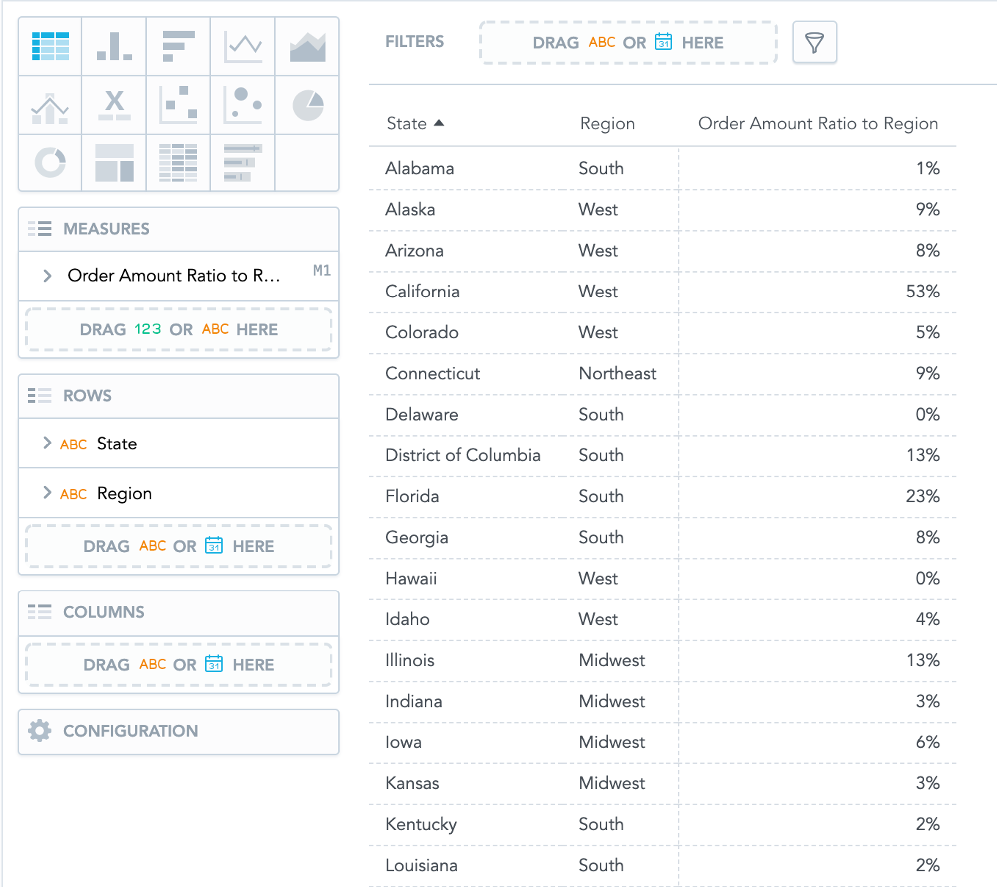
If we add our metric to the report with the Region and State dimension, we get this:

Note that the created metric displays the same reusability capabilities as the metric included here, even though it’s defined over a more straightforward LDM.

Logical Normalization

As stated above, our LDM has an implicit (non-expressed) relation between Region and State. However, we were still able to create a valuable and reusable metric computing ratio between States and Regions. There are two problems here, though:

1. We always have to include Region in our report even though it's unnecessary from the semantics perspective.
2. More importantly, we don’t have the explicit 1:N relation (between Region and State) specified in the LDM, and we must simulate it in the metric using the BY {label/region}, ALL {label/state}) construct. It means extra mental effort for the metric creators. Also, it ultimately leads to logic duplication because you have to simulate the relation in each metric where the property has to be utilized.

We would eventually like to have a new metric that would remedy our issues — in other words, it would present expected results when the report has just one attribute State, even though it’s no longer hardcoded in the metric.

To do that, we have to encode the State-Region relation into the LDM. MAQL is smart enough to recognize the situation when attributes from report and attributes from BY are from the same hierarchy. MAQL replaces the report attributes with the BY attributes — it computes both parts of the metric on different dimensionalities and automatically joins them together.

Currently, the only way to specify attributes hierarchy in the GoodData LDM is to normalize the physical database. (In the future, we plan to improve the situation via so-called logical hierarchies.)

We will extract the State-Region attributes/columns to a separate dataset/table and connect it to Order Lines via State foreign key. Here’s a simple transformation SQL script performing the denormalization of the source data:

CREATE TABLE states AS (SELECT DISTINCT state, region FROM order_lines);
ALTER TABLE states ADD CONSTRAINT pk_states PRIMARY KEY ("state");
ALTER TABLE order_lines ADD CONSTRAINT fk_order_lines_state FOREIGN KEY ("state") REFERENCES "states" ("state");
ALTER TABLE order_lines DROP COLUMN region;

To execute it, log in to the PostgreSQL database embedded in your running GoodData.CN using the following command:

psql -h localhost -p 5432 -d demo -U demouser --password

It will ask you for a password, and it is the same one that you used during the data source registration: demopass. Before you execute the SQL script, set the search path to the correct schema demo_denormalized:

SET search_path TO demo_denormalized;

You can now just copy and paste the SQL script and then go to the tab Data, where you should scan the physical database again. Do not forget to select Replace the existing model:

You should end up with the following model:

Let’s now create the new metric Order Amount Ratio to Region 2:

SELECT (SELECT SUM({fact/price})) / 
(SELECT SUM({fact/price}) BY {label/region})

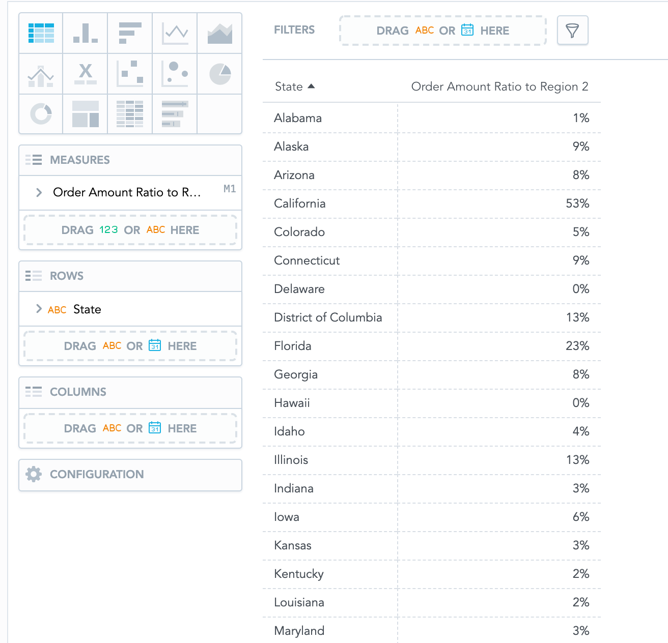
We can now add the created metric to report and remove the Region. You see that it works great with just State while also keeping the reusability aspects. (Try putting another attribute to the report, such as Product, Date, etc.)

Unfortunately, it does not work correctly if we want to compare Customers (instead of States) order amount to their Regions, even though Region is functionally dependent on the Customer (via State).

We already know how to fix that, though: explicitly express the Customer-State-Region hierarchy by changing the physical database model.

CREATE TABLE customers AS (SELECT DISTINCT customer_id, customer_name, state FROM order_lines);
ALTER TABLE customers ADD CONSTRAINT pk_customers PRIMARY KEY ("customer_id");
ALTER TABLE order_lines DROP CONSTRAINT fk_order_lines_state;
ALTER TABLE order_lines ADD CONSTRAINT fk_order_lines_customer_id FOREIGN KEY ("customer_id") REFERENCES "customers" ("customer_id");
ALTER TABLE customers ADD CONSTRAINT fk_customers_state FOREIGN KEY ("state") REFERENCES "states" ("state");
ALTER TABLE order_lines DROP COLUMN customer_name;
ALTER TABLE order_lines DROP COLUMN state;

You should scan the physical database again. Do not forget to select Replace the existing model. The result should be following:

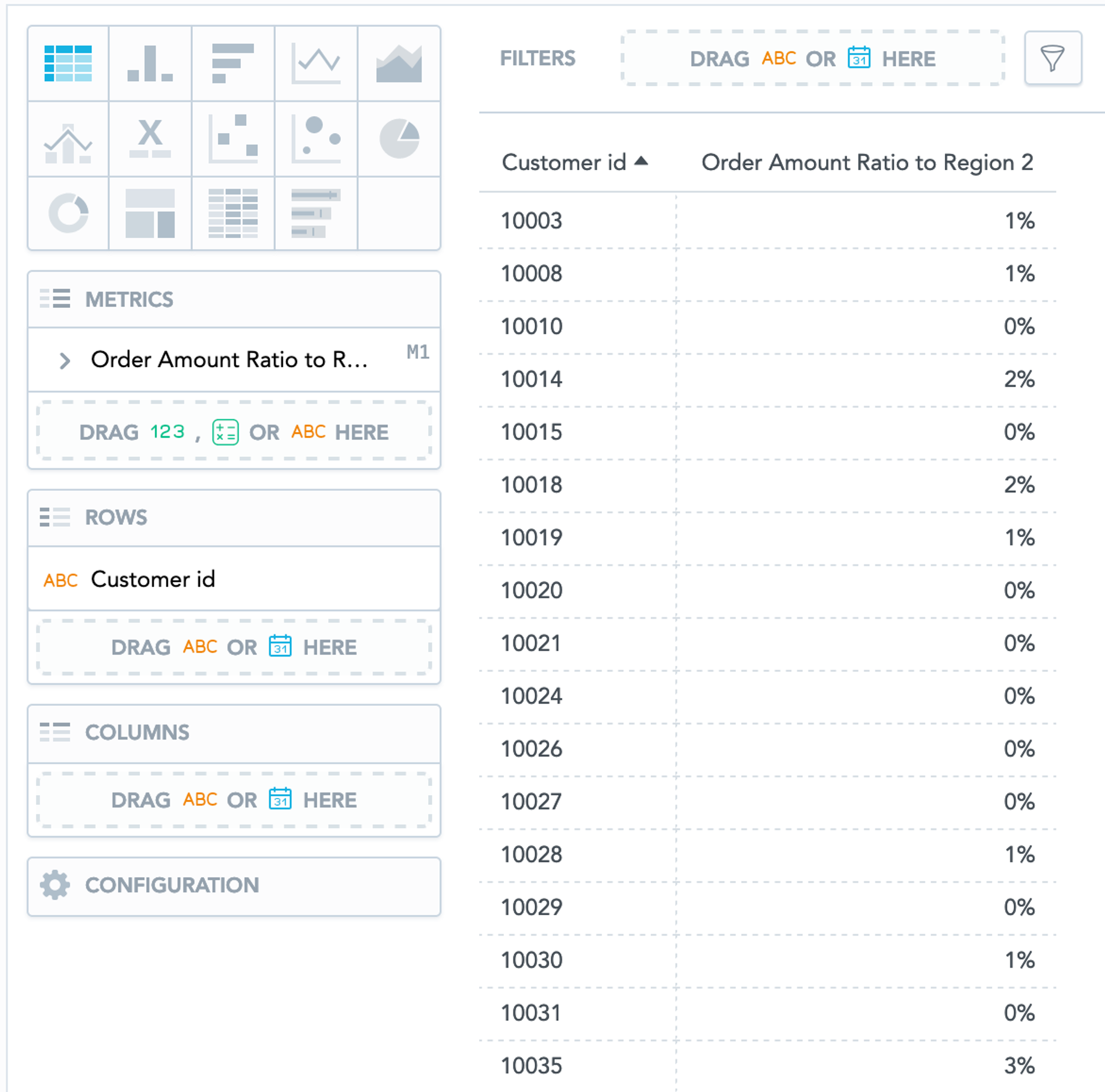
Now the Order Amount Ratio to Region 2 metric finally works as expected; it allows us to produce the following report only with the Customer id attribute.

Also, note one important advantage of abstracting your database tables to an LDM. Our metrics kept working even after we repeatedly changed the database schema and corresponding LDM.

Summary

The article described the benefits of LDM techniques to obtain valuable and reusable metrics. Still, our improved demo model is not optimal yet — we can’t answer all possible questions. Stay tuned for the second part.

Learn More About MAQL

Meanwhile, if you want to learn more about the GoodData LDM and MAQL, check our GoodData University courses. Also, see our community forum and community Slack channel for help and further info.

If you are interested in GoodData.CN, please contact us. Alternatively, sign up for a trial version of GoodData Cloud: https://www.gooddata.com/trial/

Header photo by John Schnobrich on Unsplash